Digital image correlation (DIC) is a surface displacement measurement technique that can capture the shape, motion, and deformation of solid objects. Rudimentary DIC results are easy to obtain, but reliable, high-quality DIC results can be difficult to achieve. The goal of digitalimagecorrelation.org is to equip new DIC practitioners with the basics of DIC so they can produce optimum measurements in a time-efficient manner. As a follow-on to this brief website, readers are strongly encouraged to continue their study of DIC with the “Good Practices Guide for Digital Image Correlation” from the International DIC Society.

The content of digitalimagecorrelation.org is organized for DIC learners to gather the most important information by reading from start to finish, while more experienced users can jump ahead to a section of interest. The subject matter is intentionally simplified to be accessible to engineers of all skill levels, including undergraduates. Mathematical definitions and derivations are avoided, but should be reviewed and understood by DIC practitioners once their basic skill level is established. At the conclusion of each section, suggestions are provided for more detailed resources.

1. DIC fundamentals

The basic operation of DIC is tracking a pattern (often called a speckle pattern) in a sequence of images. The process of a DIC experiment (illustrated below) can be divided into three steps: (1) obtain a pattern on the sample for tracking, (2) capture images of the sample during motion/deformation, and (3) analyze the images to compute the sample surface’s displacements.

DIC process

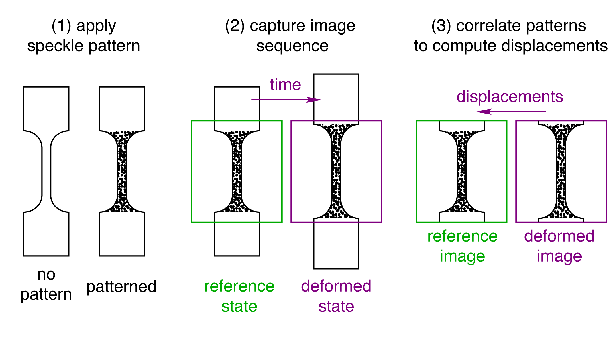
The first image in the sequence is defined as the reference image, or the baseline to which the other images are compared. DIC matches the pattern between the reference image and a deformed image, and then calculates the pattern’s displacements between the reference and deformed images.

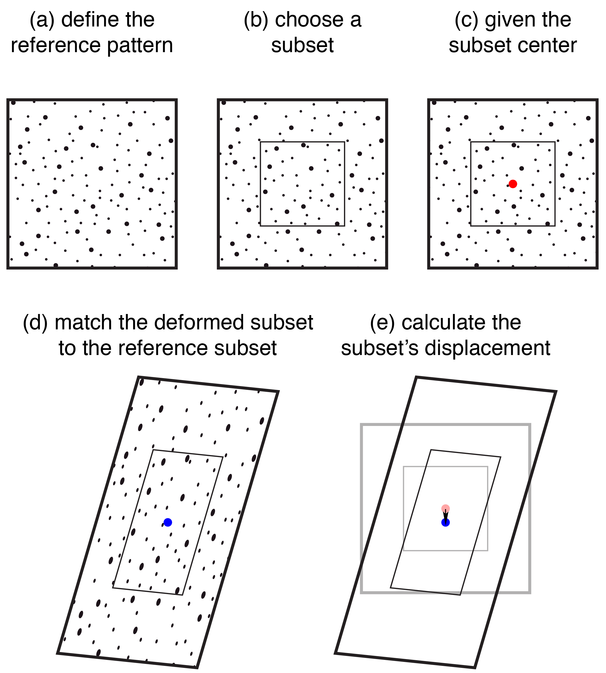
A simplification of the DIC analysis is illustrated below. (a) The reference image has a recognizable pattern of dots that will be tracked. (b) A portion of the pattern, called a subset, is selected for tracking. The term facet is also used instead of subset, but this guide adopts the term subset. (c) The center of the subset (the red dot, which is not part of the speckle pattern) is the place in the reference image from which the displacement will be calculated. (d) After the material is deformed from the reference image’s initial position, the subset in the deformed image is matched to the subset from the reference image. (e) Once the subset is matched, DIC calculates the subset center’s relative displacement between the reference and deformed images. The displacement here is the (small) difference between the blue and red dots. The next example will show how this basic operation is extended to multiple subsets and DIC points.

DIC subset

The previous example computed the displacements from one subset, but DIC computes a field of displacements by tracking multiple subsets. The same procedure as before is repeated, except this time with four equally-sized subsets in a two-by-two grid. This yields four more points with displacement information, for a total of five data points.

DIC subsets

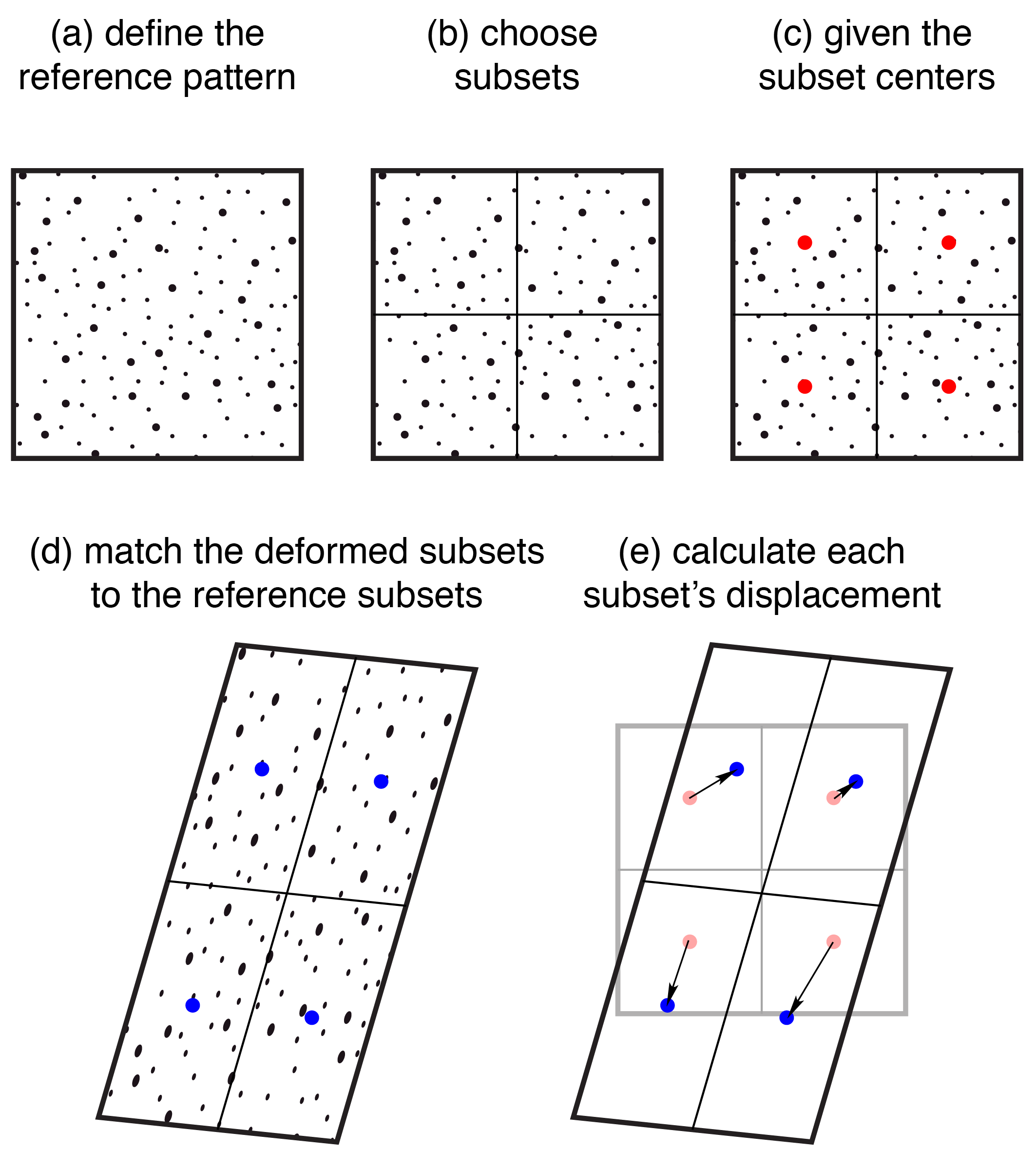
From the five subsets (one from the first example, and four more from the second example), there are five total points for which the displacements have been calculated. Each of these points can be referred to as a DIC point.

The displacement at each DIC point is a vector, so the components of the vector can be decomposed. For two dimensions of displacement, the components can be written in a Cartesian coordinate system as the horizontal displacement (u) and vertical displacement (v). Three dimensions of displacements (u, v, and w) can also be measured with a more complicated type of DIC that uses triangulation – more on this in the section on the main types of DIC.

DIC points

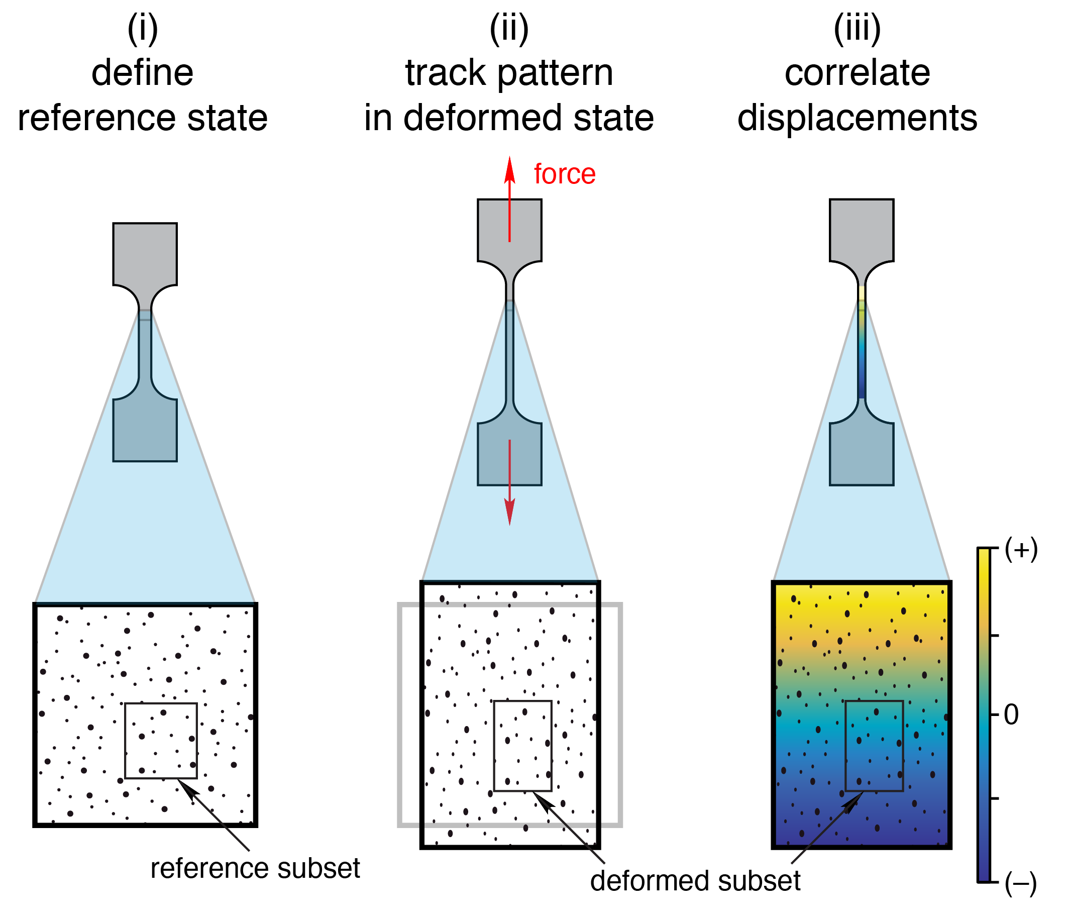
DIC is commonly utilized to study the mechanical properties of solids. One of the most common experiments for solid materials is a uniaxial tension experiment, shown in the schematic below. The goal of this experiment is to quantify how much the material deforms when a force is applied. There are many different ways to measure the deformation of the material, including strain gauges, extensometers (mechanical, laser, or optical), and DIC. While strain gauges and extensometers provide a single measurement of strain or displacement in the material, DIC can provide many displacement measurements across the material. With displacements across the material, DIC can capture the local deformations that arise from inhomogeneity, cracking, stress concentrations, plastic instabilities, phase transformations, and other localized material phenomena.

DIC basics

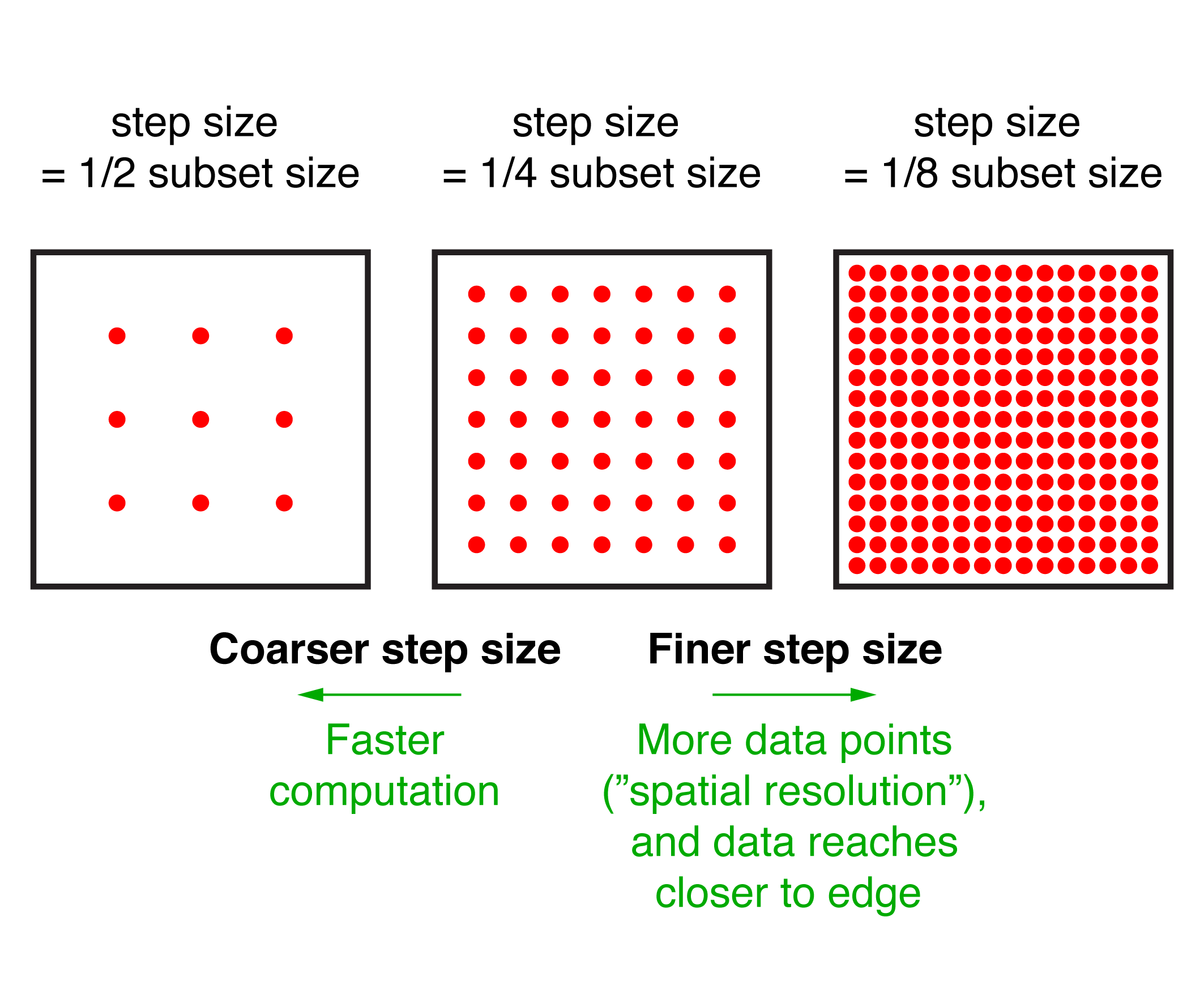
Subset and step sizes

Two important dimensions in a DIC calculation are the subset size and the step size. The subset size is the width and height of the subset square in the reference image. The step size is the distance between subset centers. Both the subset size and step size are measured in units of pixels. The most important factor for determining subset size is that each subset should contain at least three speckles (Sutton, Orteu, Schreier. doi:10.1007/978-0-387-78747-3). A secondary factor for choosing subset size is the competition of better pattern matching for bigger subsets (with more uniqueness for a larger area of features in the image) versus better spatial resolution for smaller subsets (with less spatial smoothing/filtering of the image data). A third factor is that larger subsets require more computation time. The step size has a much stronger effect on spatial resolution than the subset size. Smaller step sizes yield more DIC data points and thus higher spatial resolution. The diagram below shows a range of step sizes for the same field of view and subset sizes.

DIC setup sizes

Spatial and temporal resolution limits

Two important questions for planning DIC experiments are (1) What is the smallest displacement that this experiment can reliably measure?, and (2) What is the image exposure time that should be used?

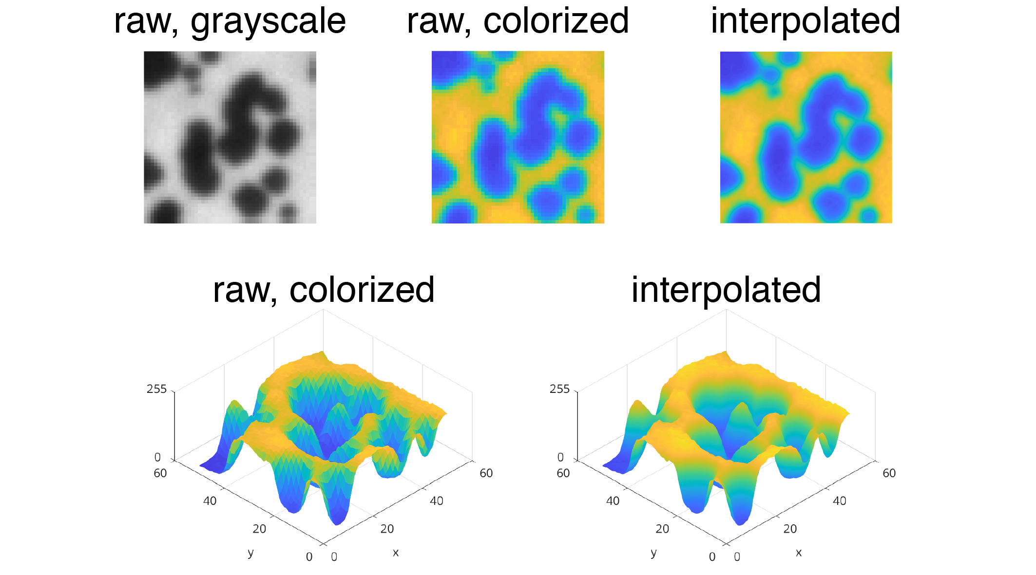
(1) The smallest possible displacement measurement is limited by the quality of the experiment’s images. In general, DIC algorithms are capable of detecting sub-pixel displacements on the order of 0.01 px. Sub-pixel displacement resolution is enabled by interpolation (generally bicubic spline interpolation) on the image data. A simple example of this interpolation is demonstrated below on a portion of an image from a DIC experiment. In practice, experimental variables introduce error into the measurements, and the smallest displacement measurements that can be expected from DIC, often called the noise floor, is on the order of

0 px.

Interpolation

(2) Since the noise floor of DIC in practice is about 0.10 px, then the images should be captured with an exposure time that limits the sample motion during the exposure time to less than 0.10 px (or even less than 0.01 px to be safe, since the theoretical limit of DIC is around 0.01 px). If the exposure time exceeded the noise floor of the calculation, then the images would have blurring that would deteriorate the DIC displacement accuracy. For example, if the sample displacement is 1 micron/second, and the imaging resolution is 10 microns/px, then the DIC noise floor is 0.10 px * (10 microns/px) = 1 micron, so the image exposure time should be less than 1 second (or less than 0.1 second to be safe, by matching the limit of 0.01 px for DIC algorithms).

Strain calculation

Computing strains is a common post-processing step with the displacements from DIC. Generally, spatial strains are computed from the displacements with a spatial derivative that has a filtering operator. This filtering in the strain calculation can blur highly-localized deformations with sharp features or discontinuities. With spatial filtering to compute the strains, the sharp features are smoothed out and can hide key phenomena like slip bands (Stinville, et al. doi:10.1007/s11340-015-0083-4).

2. Types of DIC algorithms

One way to categorize DIC algorithms is by the dimensions of the calculated displacements. For images collected by just one camera, only two dimensions of displacements can be known. This is called two-dimensional, or 2-D DIC (also commonly written as 2D-DIC). When images from more than one camera are used, depth can be measured with triangulation. This is called three-dimensional, or 3-D DIC (also commonly written as 3D-DIC).

2-D DIC assumes that the sample’s deformations are constrained to a plane that is parallel to the camera. In practice, out-of-plane motion can be a large source of error for 2-D DIC (Sutton, et al. doi:10.1016/j.optlaseng.2008.05.005). Also, images can have distortions that introduce error into DIC measurements. For example, camera lenses and optical microscopes generally have barrel distortions.

For 3-D DIC, out of plane deformations are measured with triangulation. As long as the sample remains in focus, then the out-of-plane deformations do not introduce error in 3-D DIC (unlike 2-D DIC). Furthermore, lens distortions are corrected in 3-D DIC through a calibration procedure. See the calibration section or more details about calibrating 3-D DIC systems. Another benefit of the 3-D DIC calibration process is that the length scale of the images are accurately connected to the physical length scale of the imaging system. In contrast, the length scale of 2-D DIC is introduced by a simple and less accurate conversion between the pixel size of the images to the physical size of the images (e.g. millimeters).

An important note is that 3-D DIC can only measure displacements on the surface of a material, not within the three-dimensional volume of a material. This extension of DIC from pixels to voxels (three-dimensional pixels) is called digital volume correlation (DVC). To measure displacements within a solid, the imaging system must be able to see inside the material, and the algorithms of DIC must be extended to capture displacements through the volume. Two examples of imaging systems that can see inside materials are X-ray tomography and confocal microscopy.

A comparison among 2-D DIC, 3-D DIC, and DVC is illustrated below.

DIC types

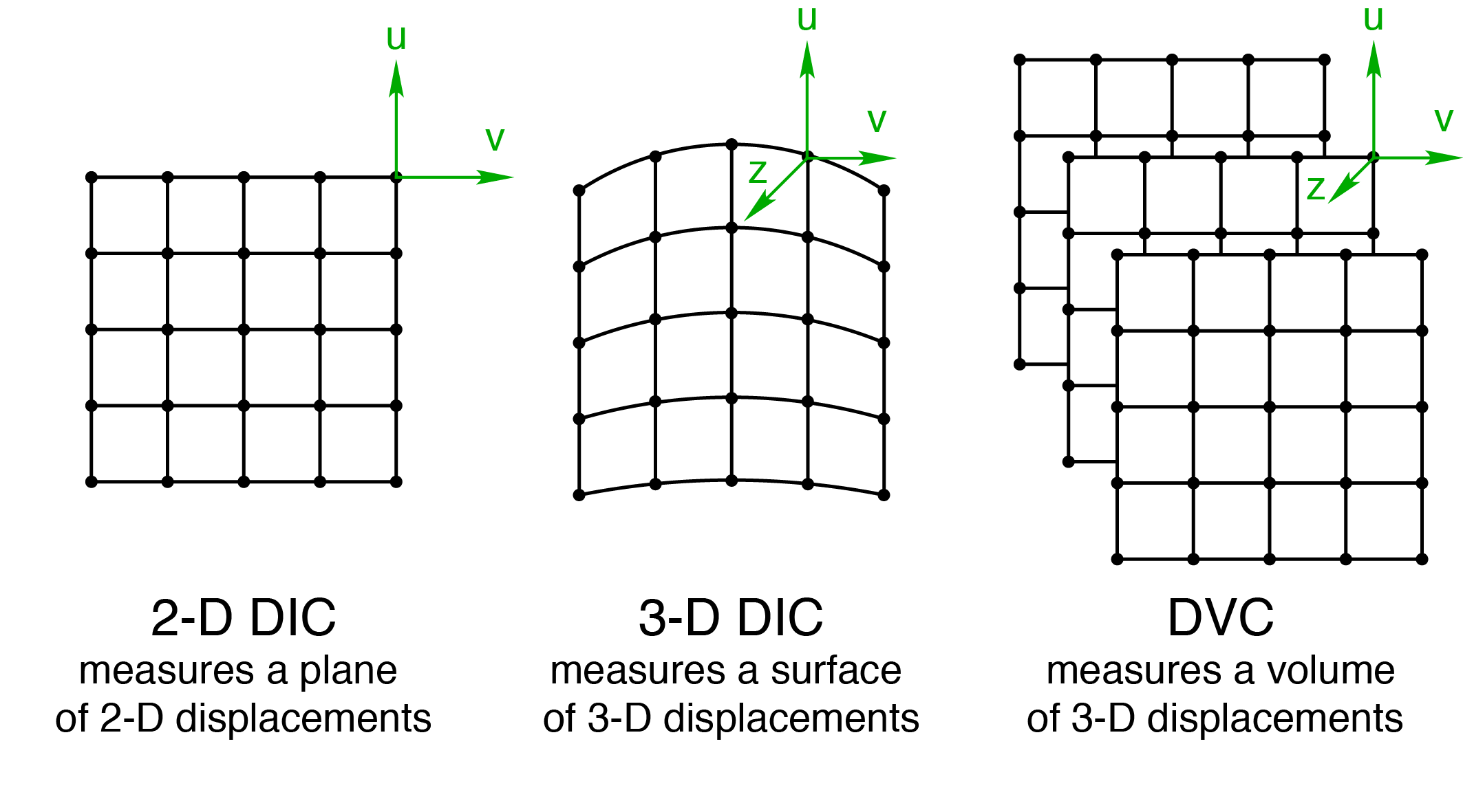
A second way to categorize DIC algorithms is by the pattern matching technique. The pattern can be separated into multiple subsets that are individually matched. This is called local DIC. Alternatively, the pattern can be matched in one go using a finite-element based approach. This is called global DIC. Local DIC was introduced before global DIC, and local DIC is more popular. Many of the principles in this guide apply to both local and global DIC, but details that only apply to local DIC (such as subsets) are included.

3. Speckle patterning

To match the reference and deformed images, DIC tracks features on the sample surface that collectively form the speckle pattern. Occasionally, a sample’s surface will inherently have features that suffice for a natural speckle pattern, but typically an artificial speckle pattern must be applied to the sample. The quality of DIC results are strongly dependent on the speckle pattern, and optimum speckle patterns meet the following conditions.

The pattern covers the sample surface in the area of interest.
The features that comprise the pattern (the speckles) are random in position but uniform in size.
The pattern moves and deforms with the sample, but does not exert a significant mechanical stress on the sample. In other words, the pattern is fully adhered to the sample, but deforms extremely easily compared to the sample. Although deformable speckles are ideal, the speckles can be rigid features that move with the sample’s deformation but do individually deform with the sample. The use of rigid speckles instead of deformable speckles adds relatively small errors to a DIC calculation (Barranger, et al. doi:10.1111/j.1475-1305.2011.00831.x).
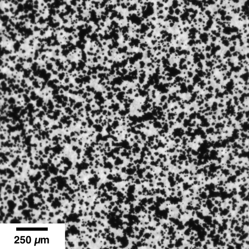
The speckle size is at least 3-by-3 pixels to avoid aliasing (Reu. doi:10.1111/ext.12111), but not much more than 7-by-7 pixels to achieve a relatively high density of DIC points (Reu. doi:10.1111/ext.12110). If speckles are much larger than 7-by-7 pixels, then there will be relatively few DIC data points possible. Also, note that these speckle sizes are not averages, but are rather the range of the smallest and largest speckles (Reu. doi:10.1111/ext.12110). Here is an example of a calculation to estimate the desired speckle size range: 12 mm / 2048 px * (3 to 7 px per speckle) = 18 to 41 microns per speckle.
The pattern has good grayscale contrast, which reduces error (Sutton, Orteu, Schreier. doi:10.1007/978-0-387-78747-3). One way to visualize this contrast is a histogram: with the number of pixels plotted with respect to grayscale level, the pattern has a mix of dark and bright pixels, indicated by two peaks in the histogram’s spectrum, and the separation between the two peaks is broad. Ideally, the two peaks look like a bimodal Gaussian distribution.
The edges of the speckles are softened (rather than sharp and distinct with the background). This allows the pixels of the camera sensor to avoid aliasing the speckle edge (Reu. doi:10.1111/ext.12139).
The pattern is stable in the testing environment. For example, for a high-temperature experiment, the pattern does not decay or darken under heating.
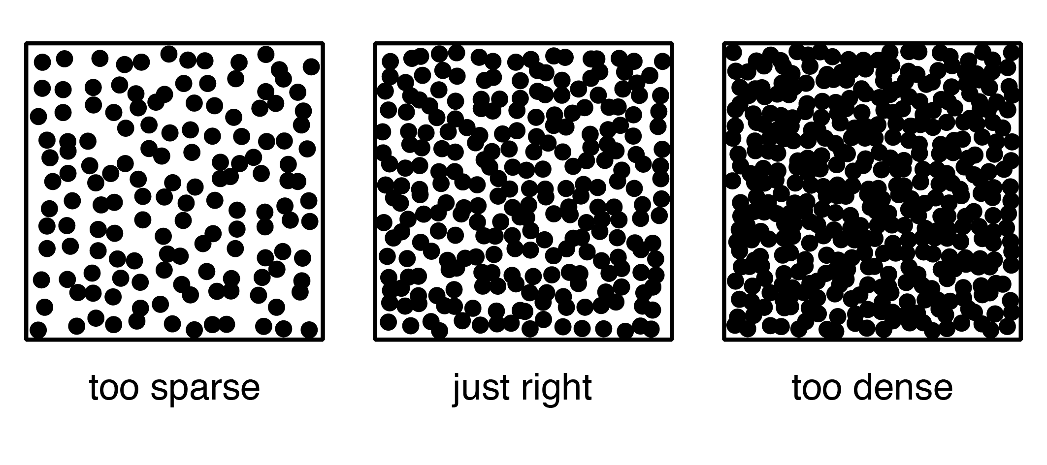
The pattern has a speckle density of about 50%. When the pattern has either too few or too many speckles, then this results in features that are both too big and too small (Reu. doi:10.1111/ext.12110). This concept is illustrated below. The artificial speckle patterns were generated with the Speckle Generator software from Correlated Solutions, Inc.

Speckle densities

Speckle patterning methods

In most cases, the sample’s natural surface is not the best pattern that could be achieved. There are many ways to apply artificial speckle patterns, and the main techniques are listed below.

Paint

Painted speckle patterns are popular because paint is relatively compliant to most engineering materials, and high-quality speckle patterns can be applied quickly with spraying paint. Since paint colors other than black and white will inherently have less contrast, black and white paints are recommended. Using white paint as the background and black as the speckles is favored over the converse order because black paint maintains better contrast over white paint (LePage, Shaw, Daly. doi:10.1007/s40799-017-0192-3).

If the sample will undergo large deformations and/or high strain rates, then plan to perform the experiment within 24 to 48 hours of painting. As the paint dries and hardens, it loses its ability to deform with the sample (Reu. doi:10.1111/ext.12147). A range of speckle sizes can be produced with sprayed paint. Artist grade airbrushes, such as the Iwata CM-B, can produce speckle sizes between 10 and 100 microns by varying the airbrush pressure (more pressure creates smaller speckles). Cans of spray paint can produce larger speckles, in the range of 100 to 1000 microns.

Inks and dyes

For hyperelastic materials (including many elastomers, polymers, and biomaterials), paint is not stretchy enough to track with the sample as a speckle pattern. Inks and dyes that permeate the sample material can be viable speckle pattern options. Stamping, masking, spraying, and stenciling can be deployed to apply the ink or dye. For example, biological soft tissue can be stained with methylene blue and then airbrushed with white paint for speckles (Lionello, et al. doi:10.1016/j.jmbbm.2014.07.007). Some DIC practitioners use permanent markers, as well.

Powder particles

For moist or sticky materials, such as silicone-based rubbers, powder particles may adhere better than paint. Graphite powder is popular for dark speckles. Alumina, talc, or magnesium oxide can be used for a white basecoat. Another use for powder patterns is achieving smaller speckles than painted patterns can produce. Using a combination of filters and compressed air, powder particle patterns smaller than 10 microns can be deposited on a smooth/polished sample to form a speckle pattern (Jonnalagadda, et al. doi:10.1007/s11340-008-9212-7).

Laser engraving

In some cases, the sample surface can be engraved with laser cutter. This method provides patterns that can remain intact during high-temperature tests (Hu, et al. doi:10.1007/s40799-018-0256-z).

Nanoparticles

For even smaller speckles than powders (about 20 to 100 nanometer speckle size, for scanning electron microscopy digital image correlation), self-assembled nanoparticles can be utilized (Kammers and Daly, doi:10.1007/s11340-013-9734-5).

Lithographed patterns

Lithography is another method for achieving small speckle size, with the benefit of a higher degree of control than most other microscale patterning methods (Cannon, et al. doi:10.1007/978-3-319-51439-0_34).

Speckle pattern gallery

To illustrate some of these concepts about speckle patterns, here are examples.

First, this is a carbon fiber that has been speckled with gold nanoparticles, following the method of Kammers and Daly (doi:10.1007/s11340-013-9734-5). Recall that a pattern should have random positions of uniformly-sized speckles. This pattern accomplishes both of these goals pretty well. The nanoparticles are all about 50 nanometers in diameter and positioned randomly. However, there are occassional clumps of nanoparticles that would detract slightly from the correlation quality.

Example nanoparticle speckle pattern on carbon fiber

Second, this is an airbrush-painted speckle pattern on a metal sample. There is good randomness in the speckle positions, but unlike the nanoparticle pattern above, this painted pattern suffers from non-uniform speckle size. Some of the speckles are too large (much larger than 7 pixels in diameter) and others are too small (less than 3 pixels in diameter). Nonetheless, this pattern would likely still correlate and produce results, albeit with less spatial resolution than possible for given the field of view.

Example paint speckle pattern on metal sample

4. Image capturing

The key step of data collection for DIC is capturing images. In general, good photography or microscopy practices translate to good DIC images, but there are extra considerations for optimizing DIC results.

The first consideration is selecting the appropriate image magnification. The image magnification depends on the length scale of the samples and phenomena that the experiments will investigate. The algorithms for DIC are inherently length scale independent, so the physical length scale conversion arises from the image magnification. For example, DIC has been performed on the length scale of meters to track the collapse of Mount St. Helens (Walter. doi:10.1130/G32198.1), all the way down to single atoms with transmission electron microscopy (Wang, et al. doi:10.1115/1.4031332). Most commonly, though, cameras are used to capture DIC images.

Building a successful DIC setup requires making the right equipment choices. For optical DIC systems with cameras, lenses, and lights, there are a few selection criteria that optimize the system.

Tips on cameras, lenses, and lights

For DIC images, color is superfluous and can be problematic. The best practice is to select black-and-white cameras. Often, cameras that are marketed for machine vision applications are very suitable for DIC, as well.
The camera sensor should have low noise, high quantum efficiency, and high dynamic range. Historically, charge-coupled device (CCD) sensors have outperformed complementary metal–oxide–semiconductor (CMOS) sensors, but new advancements in sensor technologies have leveled the playing field between CCD sensors and the next-generation of CMOS sensors (e.g. Sony Pregius).
Lenses should have low distortion. The best lenses for DIC are telecentric, which means that the sample’s magnification does not vary within the lenses depth or field of view.
For lenses with adjustable apertures, use the mid-range apertures, say f/5.6, f/8, or f/11 for an f/1.8 to f/22 lens (the more extreme apertures introduce more distortions in the imaging).
The lenses and cameras should be rigidly mounted on an optics table (ideally) or on a high-quality tripod, and sources of vibration should be minimized. Be sure to clamp, tie, or tape down the camera cables, too.
For systems with two or more cameras, much sure the cameras are viewing the same area. Small differences between the height of the epipolar lines can make calibration difficult (Reu. doi:10.1111/ext.12083).
Good focus is critical. Make sure that the most important region in your area of interest is the best-focused area.
Lighting should be evenly distributed along the sample’s area of interest. The lighting should be intense enough to achieve sufficient exposure for the images, yet not too intense to introduce saturated pixels. A saturated pixel is the maximum value of the sensor (such as 255 for an 8-bit sensor, 255 = 2^8-1). When a pixel saturates, DIC can no longer perform sub-pixel interpolation at that pixel.
The lighting should also avoid introducing too much heat. Halogen lamps are very bright but also very hot, while LEDs are cooler (but high-intensity LEDs can still generate a significant amount of heat).
For maximizing optical DIC results, polarizing filters can be placed orthogonally on the lights and lenses (a photography trick called cross polarization). For DIC, cross polarization increases contrast, decreases error, and attenuates saturated pixels that prevent sub-pixel correlation (LePage, Daly, Shaw. doi:10.1007/s11340-016-0129-2).
Lastly, using a fan to gently blow air over the DIC setup is pragmatic because the turbulent flow prevents heat waves from distorting the images (Jones, Reu. doi:10.1007/s11340-017-0354-3).

Best practices for cleaning cameras

The lenses and cameras must be cleaned to remove dust. Two easy ways to check for dust on DIC gear:
- Shine a flashlight on the lens or sensor cover and move the flashlight around at different angles. Any specks of dust will be more visible.
- Point the camera at a uniform, diffuse, bright light (e.g. light panel with a diffuser) and increase the exposure just until the image is mostly saturated, then moving the camera and seeing and darker spots in the view that don’t move while you’re moving the camera.
Be especially careful while cleaning cameras, lenses, and sensors (only clean sensors with protective covers or panels), because improperly cleaning the gear can introduce permanent scratches. For a primer on cleaning photography gear, B&H photo has a great guide.
To remove dust, do not blow air at the lenses from an air can or from your mouth, which can introduce moisture on the lens that leaves a residue. Use a photography type duster instead.
If the duster doesn’t get everything, then escalate to lens cleaning tissues. Only use new, clean lens cleaning tissues that have been moistened with lens cleaning solution.

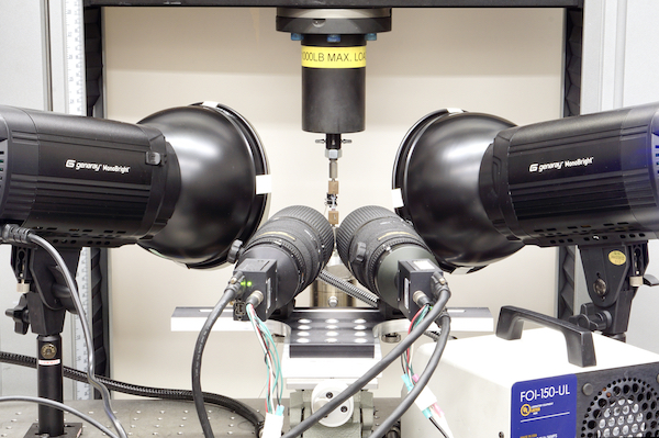
DIC setup example

An example of a 3-D DIC system is shown below. There are two cameras with two lenses, two lights in stereo with the cameras (larger lights), and another fiber optic light for back-lighting the glass calibration grid. Note the tensile sample in the mechanical testing frame has a mechanical extensometer on its gauge section. Also, there is a fan outside of the image for gently blowing air between the cameras and the sample to minimize heat waves, following Jones and Reu (doi:10.1007/s11340-017-0354-3).

DIC example setup

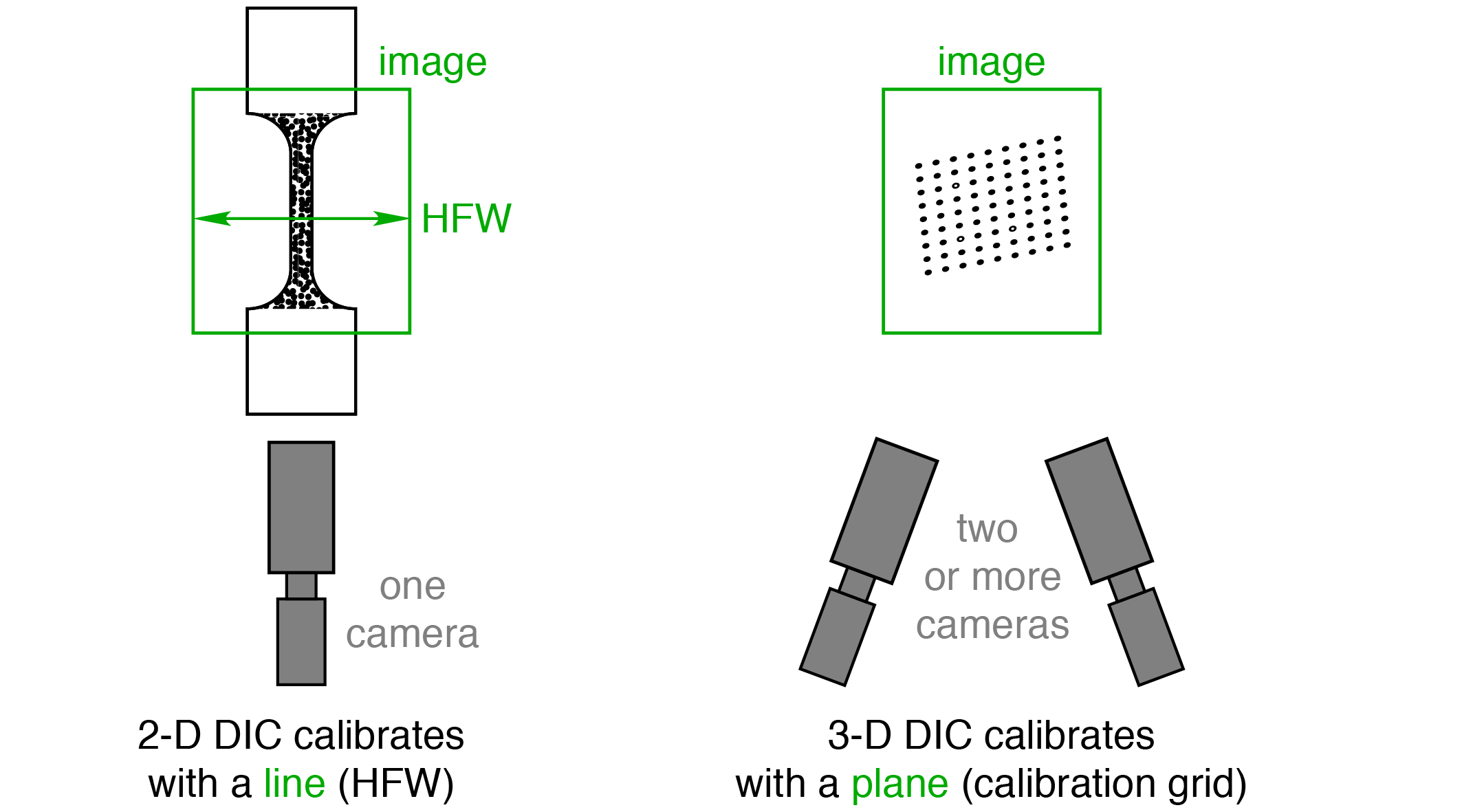
5. Calibration

For 2-D DIC, the only calibration is a length scale conversion from the pixel space of DIC to the image’s magnification, so the calibration needs a line of known length (such as the horizontal field width, or HFW). For 3-D DIC, the cameras must be calibrated with respect to one another in space, so a line is no longer sufficient. Thus, common calibration procedures involve a calibration grid, or a plane of known dimensions. This concept is illustrated below. The artificial speckle pattern and mock calibration grid were generated with the Speckle Generator and Target Generator softwares from Correlated Solutions, Inc.

DIC calibrations

For the line length measurement to calibrate 2-D DIC, small errors in the line length can create large errors in the resulting displacements, so an accurate reference such as a precision ruler should be used.

For 3-D DIC, the calibration procedure varies among DIC software packages, but general best-practices are listed below.

For an image horizontal field width (HFW) smaller than about 25 mm, a glass calibration grid with laser-etched marks is recommended due to the high precision at the small length scale. Printed grids on paper suffice for HFWs larger than about 25 mm. If using a printed grid on paper, then firmly affix the printed grid to a flat and rigid substrate, such as a section of PMMA sheet.
For glass calibration grids, backlight the grid either with a diffuse LED light panel or with indirect backlighting. One indirect backlit option is shining a light on a white poster board with a matte finish.
With the grid in the cameras, set the light intensity to just before saturation to get good contrast.
Incrementally move and rotate the grid in the field of view, then take an image pair.
Take 25-50 calibration images (more can produce even better results, but with diminishing returns).
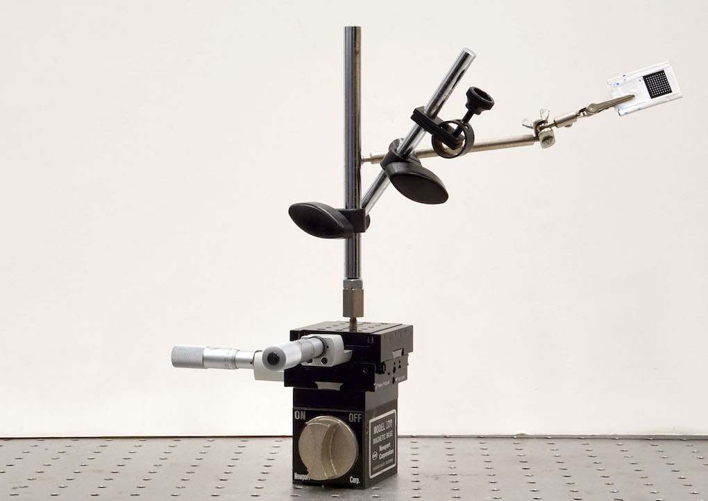
To hold the calibration grid, a dial indicator arm mounted on a two-axis stage with a magnetic base is fantastic. A lower-cost option with similar effect is a third-hand. An example of this hardware is shown below.

DIC grid holder

6. Validation and error evaluation

An important question for a DIC practitioner to ask is, “How accurate are these measurements?” Evaluating DIC errors is important because DIC results can vary widely among setups, speckle patterns, correlation parameters, and other conditions. It is difficult to separate the relative contributions of individual error sources in DIC experiments, but the overall error of an experiment can be estimated with appropriate measurements. Two possible validation and error evaluation methods are discussed below.

Measure the noise floor of the setup and speckle pattern by capturing the “Type A” errors from repeated, static images (no motion or deformation between images). The mean and distribution of the displacements represent the noise floor (which should be between about 0.01 and 0.1 px; it is not zero because of noise and error). (Reu, doi:10.1007/978-3-319-22446-6_24).
Compare the displacements (or strains) from DIC with a second measurement. A direct comparison with displacements can be accomplished with precise rigid body translations on the sample from a trusted source (e.g. Vernier micrometer or precision linear stage). The displacements can also be measured from an LVDT, laser, or other techniques. Strains and deformations can be compared with extensometers (mechanical or laser), as well as strain gauges (although strain gauges are limited to small strains).

digitalimagecorrelation.org

1. DIC fundamentals

Subset and step sizes

Spatial and temporal resolution limits

Strain calculation

Further reading

2. Types of DIC algorithms

Further reading

3. Speckle patterning

Speckle patterning methods

Paint

Inks and dyes

Powder particles

Laser engraving

Nanoparticles

Lithographed patterns

Speckle pattern gallery

Further reading

4. Image capturing

Tips on cameras, lenses, and lights

Best practices for cleaning cameras

DIC setup example

Further reading

5. Calibration

Further reading

6. Validation and error evaluation